Basic usage¶

Attention

The basic usage setup has limited functionality and omits many features in favor of a quick-start setup. To leverage the full functionality of GERBLS, see Full usage.

Overview¶

The basic usage version of GERBLS is designed to be a quick-start alternative to astropy.timeseries.BoxLeastSquares.autopower(). It is implemented via a wrapper function gerbls.run_bls() that returns a dictionary containing the generated BLS spectrum:

gerbls.run_bls(time, mag, err, min_period, max_period, durations, t_samp=0.0)[source]

A basic convenience function to generate a BLS spectrum. The input data will be resampled to a uniform time cadence to run the BLS, use t_samp to explicitly provide the cadence for resampling. Automatic downsampling will be used to maintain an optimal period spacing.

Parameters:

time (ArrayLike) – Array of observation timestamps.

mag (ArrayLike) – Array of observed fluxes.

err (ArrayLike) – Array of flux uncertainties for each observation.

min_period (float) – Minimum BLS period to search.

max_period (float) – Maximum BLS period to search.

durations (list or float) – List of transit durations to test at each period.

t_samp (float, optional) – Time sampling to bin the data before running the BLS. If 0 (default), the median time difference between observations is used.

Returns:

A dictionary with BLS results:

Key

Value

P

list of tested periods

dchi2

BLS statistic (\(\Delta\chi^2\)) at each period

t0

best-fit transit mid-point at each period

dur

best-fit duration at each period

mag0

best-fit flux baseline at each period

dmag

best-fit transit depth at each period

snr

estimated SNR at each period

Return type:

dict

Key	Value
`P`	list of tested periods
`dchi2`	BLS statistic (\(\Delta\chi^2\)) at each period
`t0`	best-fit transit mid-point at each period
`dur`	best-fit duration at each period
`mag0`	best-fit flux baseline at each period
`dmag`	best-fit transit depth at each period
`snr`	estimated SNR at each period

time, mag, and err will be coerced into NumPy arrays and sorted in time (if needed). If the flux uncertainties are homoscedastic (equal for all data points), err should still be passed as an array filled with equal values, with the same length as time and mag. durations can be passed as a single value, to test a single transit duration across all periods.

The fast-folding BLS requires data to be evenly spaced in time. gerbls.run_bls() provides an optional parameter t_samp that can be used to resample (bin) the data to the required cadence before running the BLS. Increasing this value will make the BLS run faster; however, one should make sure that any real transits in the data are at least a few times larger than the value for t_samp so they do not get removed by the binning. If no value is provided for t_samp, the median time sampling of the input data is used: this works well if the input time array is already close to evenly sampled.

Important

Changing t_samp has a large effect on BLS runtime speed as well as the number of orbital periods tested. To test fewer periods and make the BLS run faster, increase the value of t_samp. See The period grid for more info.

We note that the light curve should already be detrended for systematics and stellar variability prior to running the BLS. You may use any of your favorite detrending algorithms. For long-term variability, the Savitsky-Golay filter is a relatively good starting point - see gerbls.clean_savgol() or scipy.signal.savgol_filter().

Example¶

Given input data arrays time, mag, and err, the following code generates a BLS spectrum for orbital periods between 0.4 and 10 days (assuming that time is in days). At each period, it tests transit durations of 1 and 2 hours. The time sampling t_samp is not specified explicitly, so it is set to the median time sampling of the input data (time).

>>> from gerbls import run_bls
>>> results = run_bls(time, mag, err, 0.4, 10., [1./24, 2./24])

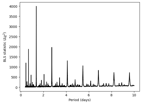
The resulting BLS spectrum can then be plotted as follows (a sample data set has been used to generate the plot below):

>>> import matplotlib.pyplot as plt
>>> plt.plot(results['P'], results['dchi2'], "k-")
>>> plt.xlabel("Period (days)")
>>> plt.ylabel("BLS statistic ($\Delta\chi^2$)")
>>> plt.show()

For additional customization options while running the BLS, as well as convenient tools to identify peaks in the BLS periodogram, see Full usage.