Fast BLS demonstration

This page demonstrates the functionality of GERBLS by applying a fast-folding BLS to a simulated data set. First, we set up the necessary imports:

import gerbls
import matplotlib.pyplot as plt
import numpy as np

The data set we are using is included in the GERBLS source distribution as tests/phottest.dat. It includes a simulated transit with a period of 1.37 days. In order to run GERBLS, we need to store the data in a gerbls.pyDataContainer object.

phottest = np.loadtxt("../../../tests/phottest.dat")
time, mag, err = phottest.T

data = gerbls.pyDataContainer()
data.store(time, mag, err)

plt.figure(figsize=(12, 6))
plt.plot(data.rjd - 2400000.5, data.mag, ".")
plt.xlabel("Time (JD - 2400000.5)")
plt.ylabel("Flux")
plt.show()

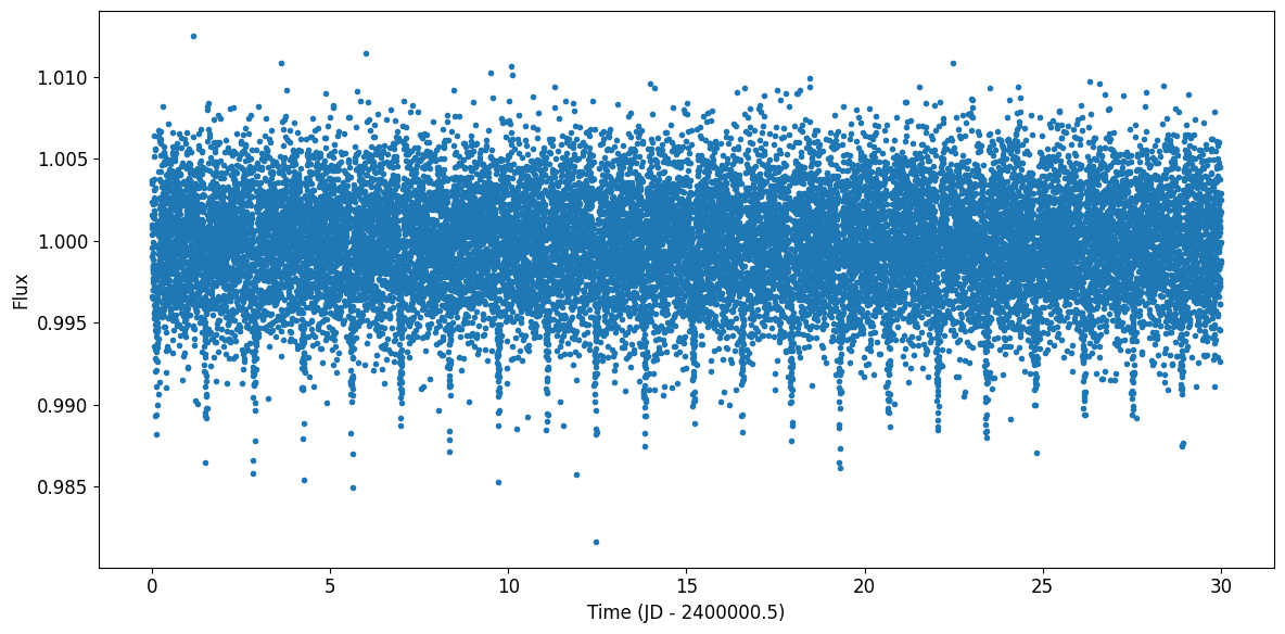
It should be noted that any long-term trends in the data (due to stellar variability, instrument systematics, etc.) should be subtracted from the data via detrending before running the BLS. GERBLS provides a wrapper on a Savitsky-Golay filter via gerbls.clean_savgol(), which can handle basic long-term variability; however, more complex detrenders may be required for some data sets. In this example data set, there is no long-term stellar variability, so we shall just use data as our detrended data.

Next, we can set up the fast-folding BLS.

min_period = 0.4    # Minimum searched orbital period (in days)
max_period = 10.    # Maximum searched orbital period (in days)
t_samp = 10./60/24  # Desired time sampling of the data

bls = gerbls.pyFastBLS()
bls.setup(data,
          min_period,
          max_period,
          t_samp=t_samp,
          duration_mode='constant',
          durations=[0.5/24, 1./24, 2./24])

The time sampling (t_samp) is a key parameter of the fast-folding BLS. Before running the BLS, the data is resampled to the specified time cadence (here, 10 minutes). A shorter sampling time increases the BLS precision as well as the number of periods searched, but it also makes the BLS run slower. Thus, when speed is important, t_samp can be cautiously increased as long as its value remains substantially below the expected duration of the transits. If not given (t_samp is an optional parameter), its value is set to the median time cadence of the input data. In this example, we are also fitting for three different transit durations (0.5, 1, and 2 hours) at each tested period.

We can now generate the BLS spectrum, saving the results in double precision to be safe (an equivalent floating point method bls.run() is also available and runs slightly faster).

bls.run_double(verbose=True)

Starting FFA...
Downsampling: OFF
Number of tested periods: 16595
BLS runtime: 0.137918 sec

The number of tested periods was 16,595; this can be affected by changing t_samp or the range of searched orbital periods. In order to process the results of the BLS analysis, we create an instance of gerbls.pyBLSAnalyzer, which allows us to easily retrieve the \(\Delta\chi^2\) values (difference in \(\chi^2\) between a fitted box model and a constant-flux model with no transit) as well as other fitted parameters at each tested orbital period.

blsa = gerbls.pyBLSAnalyzer(bls)

plt.figure(figsize=(12, 6))
plt.semilogx(blsa.P, blsa.dchi2, "k-")
plt.xlim(blsa.P.min(), blsa.P.max())
plt.ylim(0)
plt.xlabel("Period (days)")
plt.ylabel("$\Delta\chi^2$")
plt.show()

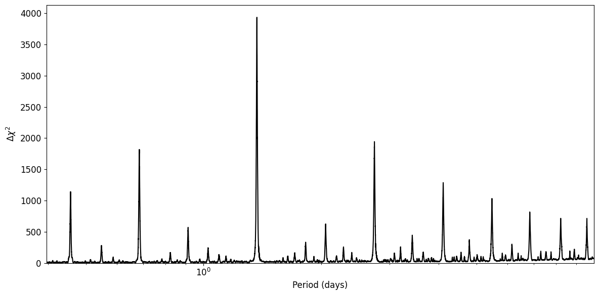
It should be noted that the SNR of each peak can be estimated from \(SNR \approx \sqrt{\Delta\chi^2}\); the array blsa.dchi2 can be replaced with blsa.snr to retrieve these values automatically. Furthermore, the BLS spectrum exhibits a small positive baseline trend as a function of orbital period. At longer periods, the number of in-transit data points decreases, which makes it more likely to obtain spuriously high values of \(\Delta\chi^2\). One way to fix this is to normalize the SNR spectrum and calculate the Signal Detection Efficiency at each period (\(SDE\), modified from Kovacs et al. 2002):

\[SDE = \frac{BLS_{peak} - BLS_{trend}}{BLS_{scatter}}\]

Kovacs et al used Signal Residue (\(SR\)) as the BLS statistic, which is proportional to \(\sqrt{\Delta\chi^2}\). GERBLS can estimate the \(SDE\) values by using a median filter to calculate \(BLS_{trend}\) (the window length can be adjusted and is equal to 1001 by default) and estimating \(BLS_{scatter}\) from the standard deviation of the residuals:

plt.figure(figsize=(12, 6))
plt.semilogx(blsa.P, blsa.get_SDE(), "k-")
plt.xlim(blsa.P.min(), blsa.P.max())
plt.xlabel("Period (days)")
plt.ylabel("$SDE$")
plt.show()

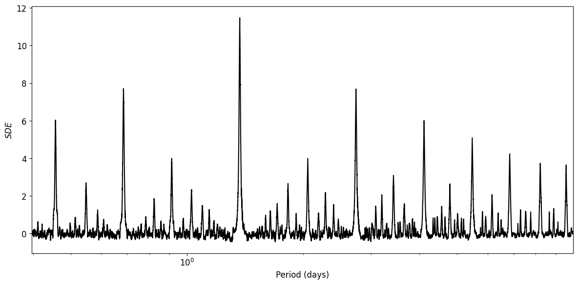
There is a clear peak close to a period of 1.4 days, corresponding to the transits in the data. gerbls.pyBLSAnalyzer provides a method called generate_models(N), which returns the parameters of the top \(N\) peaks in the BLS spectrum. Below, we just retrieve the box model corresponding to the highest BLS peak and overlay it on top of the original data phase folded to the detected orbital period.

model = blsa.generate_models(1, use_SDE=False)[0]

# Print information about the top BLS peak
print(model)

# Arrays to overlay the best-fit box model
fit_x = [0, model.t0 - model.dur / 2, model.t0 - model.dur / 2,
         model.t0 + model.dur / 2, model.t0 + model.dur / 2, model.P]
fit_y = np.array([0, 0, -model.dmag, -model.dmag, 0, 0]) + model.mag0

plt.figure(figsize=(12, 6))
plt.plot(data.rjd % model.P, data.mag, ".")
plt.plot(fit_x, fit_y, "k--")
plt.xlim(0, model.P)
plt.xlabel("Orbital phase (days)")
plt.ylabel("Flux")
plt.show()

pyBLSResult(P=1.3700425643508432, dchi2=3935.128078962631, mag0=0.9999769610443007, dmag=0.005340897349998262, t0=1.1655193456645943, dur=0.08333333333333333, snr=62.73059922368533)

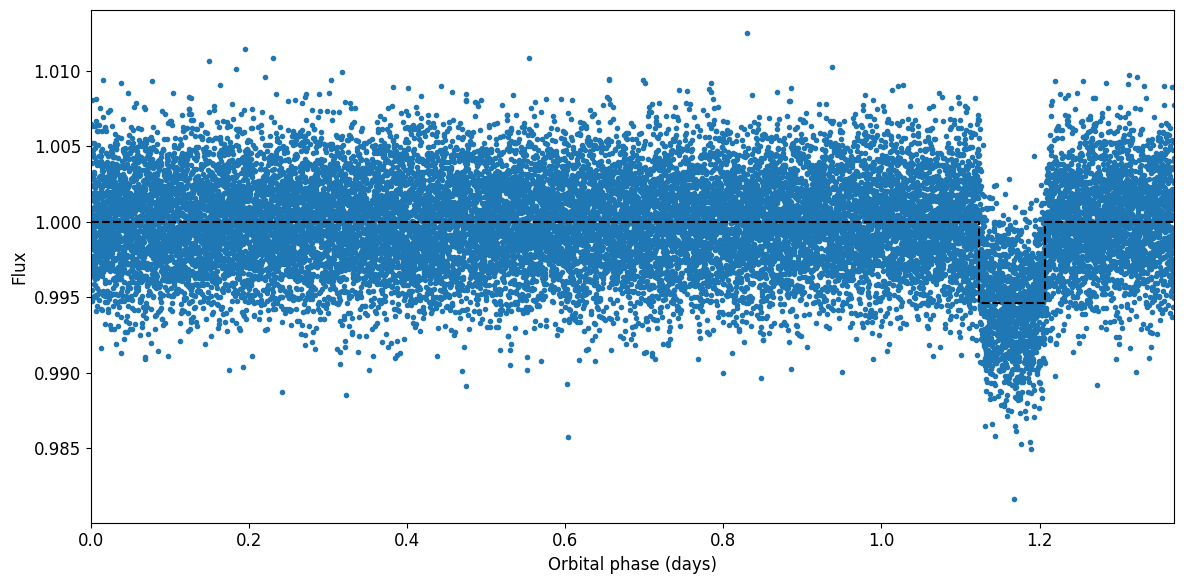
It is a clear match! Note that one of our searched transit duration (2 hours) was reasonably close to the actual transits in the data, which improves the \(\Delta\chi^2\). We can use a couple of convenience methods to retrieve an error estimate on the transit depth and use that to calculate the SNR:

print(f"Fitted transit depth: {model.dmag:.5f} +/- {model.get_dmag_err(data):.5f}")
print(f"SNR: {model.get_SNR(data):.4f}")

Fitted transit depth: 0.00534 +/- 0.00009
SNR: 62.7495

GERBLS also provides an easy way to use batman to fit for a limb-darkened transit model, with the initial guesses for the fitted parameters taken from the BLS model. We can fit for all the orbital parameters as well as the two quadratic limb darkening parameters:

model_LD = gerbls.LDModel.from_BLS(model)
model_LD.fit(data)
print(model_LD)

LDModel with the following orbital parameters:
    b = 0.000000 +/- 0.000000
 mag0 = 0.999977 +/- 0.000021
    P = 1.370043 +/- 0.000000
    r = 0.073082 +/- 0.000746
   t0 = 1.165519 +/- 0.000303
and the following stellar parameters:
   u1 = 0.328634 +/- 0.277302
   u2 = 0.219089 +/- 0.270670
    M =   1.0000
    R =   1.0000
and the following fit parameters:
 chi2 =   21593.0787 (reduced: 0.9997)
dchi2 =   4074.0089

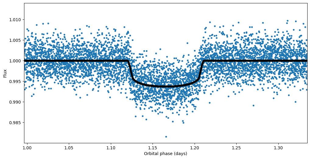
We can plot the fitted limb-darkened model (zoomed in close to the actual transit mid-point).

plt.figure(figsize=(12, 6))
plt.plot(data.rjd % model_LD.P, data.mag, ".")
plt.plot(data.rjd % model_LD.P, model_LD.eval(data.rjd), "k.")
plt.xlim(model_LD.t0 - model_LD.dur * 2, model_LD.t0 + model_LD.dur * 2)
plt.xlabel("Orbital phase (days)")
plt.ylabel("Flux")
plt.show()